The Fellegi-Sunter model¶

This topic guide gives a high-level introduction to the Fellegi Sunter model, the statistical model that underlies Splink's methodology.

For a more detailed interactive guide that aligns to Splink's methodology see Robin Linacre's interactive introduction to probabilistic linkage.

Parameters of the Fellegi-Sunter model¶

The Fellegi-Sunter model has three main parameters that need to be considered to generate a match probability between two records:

\(\lambda\) - probability that any two records match
\(m\) - probability of a given observation given the records are a match
\(u\) - probability of a given observation given the records are not a match

λ probability¶

The lambda (\(\lambda\)) parameter is the prior probability that any two records match. I.e. assuming no other knowledge of the data, how likely is a match? Or, as a formula:

\[ \lambda = Pr(\textsf{Records match}) \]

This is the same for all records comparisons, but is highly dependent on:

The total number of records
The number of duplicate records (more duplicates increases \(\lambda\))
The overlap between datasets
- Two datasets covering the same cohort (high overlap, high \(\lambda\))
- Two entirely independent datasets (low overlap, low \(\lambda\))

m probability¶

The \(m\) probability is the probability of a given observation given the records are a match. Or, as a formula:

\[ m = Pr(\textsf{Observation | Records match}) \]

For example, consider the the \(m\) probability of a match on Date of Birth (DOB). For two records that are a match, what is the probability that:

DOB is the same:
Almost 100%, say 98% \(\Longrightarrow m \approx 0.98\)
DOB is different:
Maybe a 2% chance of a data error? \(\Longrightarrow m \approx 0.02\)

The \(m\) probability is largely a measure of data quality - if DOB is poorly collected, it may only match exactly for 50% of true matches.

u probability¶

The \(u\) probability is the probability of a given observation given the records are not a match. Or, as a formula:

\[ u = Pr(\textsf{Observation | Records do not match}) \]

For example, consider the the \(u\) probability of a match on Surname. For two records that are not a match, what is the probability that:

Surname is the same:
Depending on the surname, <1%? \(\Longrightarrow u \approx 0.005\)
Surname is different:
Almost 100% \(\Longrightarrow u \approx 0.995\)

The \(u\) probability is a measure of coincidence. As there are so many possible surnames, the chance of sharing the same surname with a randomly-selected person is small.

Interpreting m and u¶

In the case of a perfect unique identifier:

A person is only assigned one such value - \(m = 1\) (match) or \(m=0\) (non-match)
A value is only ever assigned to one person - \(u = 0\) (match) or \(u = 1\) (non-match)

Where \(m\) and \(u\) deviate from these ideals can usually be intuitively explained:

m probability¶

A measure of data quality/reliability.

How often might a person's information change legitimately or through data error?

Names: typos, aliases, nicknames, middle names, married names etc.
DOB: typos, estimates (e.g. 1st Jan YYYY where date not known)
Address: formatting issues, moving house, multiple addresses, temporary addresses

u probability¶

A measure of coincidence/cardinality¹.

How many different people might share a given identifier?

DOB (high cardinality) – for a flat age distribution spanning ~30 years, there are ~10,000 DOBs (0.01% chance of a match)
Sex (low cardinality) – only 2 potential values (~50% chance of a match)

Match Weights¶

One of the key measures of evidence of a match between records is the match weight.

Deriving Match Weights from m and u¶

The match weight is a measure of the relative size of \(m\) and \(u\):

\[ \begin{equation} \begin{aligned} M &= \log_2\left(\frac{\lambda}{1-\lambda}\right) + \log_2 K \\[10pt] &= \log_2\left(\frac{\lambda}{1-\lambda}\right) + \log_2 m - \log_2 u \end{aligned} \end{equation} \]

where \(\lambda\) is the probability that two random records match and \(K=m/u\) is the Bayes factor.

A key assumption of the Fellegi Sunter model is that observations from different column/comparisons are independent of one another. This means that the Bayes factor for two records is the products of the Bayes factor for each column/comparison:

\[ K_\textsf{features} = K_\textsf{forename} \cdot K_\textsf{surname} \cdot K_\textsf{dob} \cdot K_\textsf{city} \cdot K_\textsf{email} \]

This, in turn, means that match weights are additive:

\[ M_\textsf{obs} = M_\textsf{prior} + M_\textsf{features} \]

where \(M_\textsf{prior} = \log_2\left(\frac{\lambda}{1-\lambda}\right)\) and \(M_\textsf{features} = M_\textsf{forename} + M_\textsf{surname} + M_\textsf{dob} + M_\textsf{city} + M_\textsf{email}\).

So, considering these properties, the total match weight for two observed records can be rewritten as:

\[ \begin{equation} \begin{aligned} M_\textsf{obs} &= \log_2\left(\frac{\lambda}{1-\lambda}\right) + \sum_{i}^\textsf{features}\log_2(\frac{m_i}{u_i}) \\[10pt] &= \log_2\left(\frac{\lambda}{1-\lambda}\right) + \log_2\left(\prod_i^\textsf{features}\frac{m_i}{u_i}\right) \end{aligned} \end{equation} \]

Interpreting Match Weights¶

The match weight is the central metric showing the amount of evidence of a match is provided by each of the features in a model. The is most easily shown through Splink's Waterfall Chart:

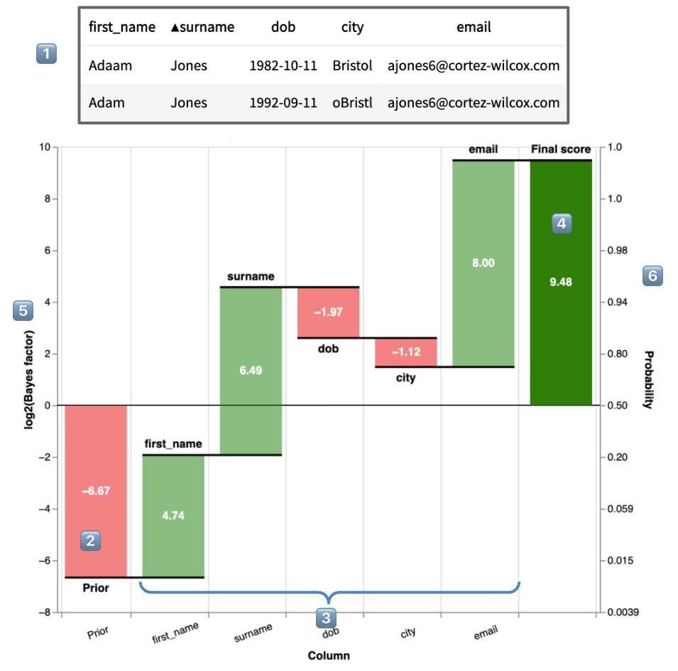
1️⃣ are the two records being compared
2️⃣ is the match weight of the prior, \(M_\textsf{prior} = \log_2\left(\frac{\lambda}{1-\lambda}\right)\). This is the match weight if no additional knowledge of features is taken into account, and can be thought of as similar to the y-intercept in a simple regression.
3️⃣ are the match weights of each feature, \(M_\textsf{forename}\), \(M_\textsf{surname}\), \(M_\textsf{dob}\), \(M_\textsf{city}\) and \(M_\textsf{email}\) respectively.
4️⃣ is the total match weight for two observed records, combining 2️⃣ and 3️⃣:

\[ \begin{equation} \begin{aligned} M_\textsf{obs} &= M_\textsf{prior} + M_\textsf{forename} + M_\textsf{surname} + M_\textsf{dob} + M_\textsf{city} + M_\textsf{email} \\[10pt] &= -6.67 + 4.74 + 6.49 - 1.97 - 1.12 + 8.00 \\[10pt] &= 9.48 \end{aligned} \end{equation} \]
5️⃣ is an axis representing the \(\textsf{match weight} = \log_2(\textsf{Bayes factor})\))
6️⃣ is an axis representing the equivalent match probability (noting the non-linear scale). For more on the relationship between match weight and probability, see the sections below

Match Probability¶

Match probability is a more intuitive measure of similarity than match weight, and is, generally, used when choosing a similarity threshold for record matching.

Deriving Match Probability from Match Weight¶

Probability of two records being a match can be derived from the total match weight:

\[ Pr(\textsf{Match | Observation}) = \frac{2^{M_\textsf{obs}}}{1+2^{M_\textsf{obs}}} \]

Example

Consider the example in the Interpreting Match Weights section. The total match weight, \(M_\textsf{obs} = 9.48\). Therefore,

\[ Pr(\textsf{Match | Observation}) = \frac{2^{9.48}}{1+2^{9.48}} \approx 0.999 \]

Understanding the relationship between Match Probability and Match Weight¶

It can be helpful to build up some intuition for how match weight translates into match probability.

Plotting match probability versus match weight gives the following chart:

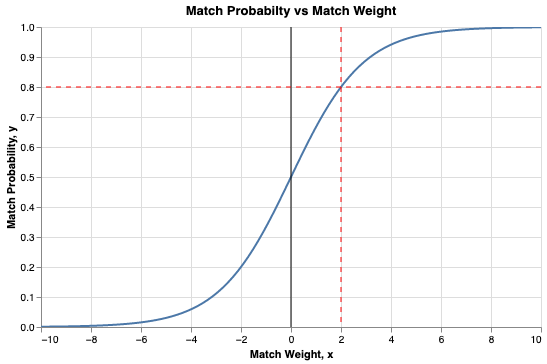
Some observations from this chart:

\(\textsf{Match weight} = 0 \Longrightarrow \textsf{Match probability} = 0.5\)
\(\textsf{Match weight} = 2 \Longrightarrow \textsf{Match probability} = 0.8\)
\(\textsf{Match weight} = 3 \Longrightarrow \textsf{Match probability} = 0.9\)
\(\textsf{Match weight} = 4 \Longrightarrow \textsf{Match probability} = 0.95\)
\(\textsf{Match weight} = 7 \Longrightarrow \textsf{Match probability} = 0.99\)

So, the impact of any additional match weight on match probability gets smaller as the total match weight increases. This makes intuitive sense as, when comparing two records, after you already have a lot of evidence/features indicating a match, adding more evidence/features will not have much of an impact on the probability of a match.

Similarly, if you already have a lot of negative evidence/features indicating a match, adding more evidence/features will not have much of an impact on the probability of a match.

Deriving Match Probability from m and u¶

Given the definitions for match probability and match weight above, we can rewrite the probability in terms of \(m\) and \(u\).

\[ \begin{equation} \begin{aligned} Pr(\textsf{Match | Observation}) &= \frac{2^{\log_2\left(\frac{\lambda}{1-\lambda}\right) + \log_2\left(\prod_{i}^\textsf{features}\frac{m_{i}}{u_{i}}\right)}}{1+2^{\log_2\left(\frac{\lambda}{1-\lambda}\right) + \log_2\left(\prod_{i}^\textsf{features}\frac{m_{i}}{u_{i}}\right)}} \\[20pt] &= \frac{\left(\frac{\lambda}{1-\lambda}\right)\prod_{i}^\textsf{features}\frac{m_{i}}{u_{i}}}{1+\left(\frac{\lambda}{1-\lambda}\right)\prod_{i}^\textsf{features}\frac{m_{i}}{u_{i}}} \\[20pt] &= 1 - \left[1+\left(\frac{\lambda}{1-\lambda}\right)\prod_{i}^\textsf{features}\frac{m_{i}}{u_{i}}\right]^{-1} \end{aligned} \end{equation} \]

The Fellegi-Sunter model¶

Parameters of the Fellegi-Sunter model¶

λ probability¶

m probability¶

u probability¶

Interpreting m and u¶

m probability¶

u probability¶

Match Weights¶

Deriving Match Weights from m and u¶

Interpreting Match Weights¶

Match Probability¶

Deriving Match Probability from Match Weight¶

Understanding the relationship between Match Probability and Match Weight¶

Deriving Match Probability from m and u¶

Further Reading¶