`profile_columns`¶

At a glance

Useful for: Looking at the distribution of values in columns.

API Documentation: profile_columns()

What is needed to generate the chart?: A linker with some data.

Worked Example¶

import altair as alt
from splink.datasets import splink_datasets
from splink.duckdb.linker import DuckDBLinker

df = splink_datasets.historical_50k
linker = DuckDBLinker(df)

linker.profile_columns()

What the chart shows¶

The profile_columns chart shows 3 charts for each selected column:

The left chart shows the distribution of all values in the column. The width of each "step" represents the proportion of all (non-null) values of a given value while the height of each "step" gives the count of the same given value.
The middle chart shows the counts of the ten most common values in the column. These correspond to the 10 leftmost "steps" in the left chart.
The right chart shows the counts of the ten least common values in the column. These correspond to the 10 rightmost "steps" in the left chart.

What the chart tooltip shows

Left chart:¶

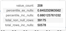
This tooltip shows a number of statistics based on the column value of the "step" that the user is hovering over, including:

The number of occurances of the given value.
The precentile of the column value (excluding and including null values).
The total number of rows in the column (excluding and including null values).

Middle and right chart:¶

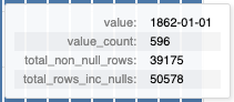
This tooltip shows a number of statistics based on the column value of the bar that the user is hovering over, including:

The column value
The count of the column value.
The total number of rows in the column (excluding and including null values).

How to interpret the chart¶

The distribution of values in your data is important for two main reasons:

Columns with higher cardinality (number of distinct values) are usually more useful for data linking. For instance, date of birth is a much stronger linkage variable than gender.
The skew of values is important. If you have a birth_place column that has 1,000 distinct values, but 75% of them are London, this is much less useful for linkage than if the 1,000 values were equally distributed

Actions to take as a result of the chart¶

In an ideal world, all of the columns in datasets used for linkage would be high cardinality with a low skew (i.e. many distinct values that are evenly distributed). This is rarely the case with real-life datasets, but there a number of steps to extract the most predictive value, particularly with skewed data.

Skewed String Columns¶

Consider the skew of birth_place in our example:

linker.profile_columns("birth_place")

Here we can see that "london" is the most common value, with many multiples more entires than the other values. In this case two records both having a birth_place of "london" gives far less evidence for a match than both having a rarer birth_place (e.g. "felthorpe").

To take this skew into account, we can build Splink models with Term Frequency Adjustments. These adjustments will increase the amount of evidence for rare matching values and reduce the amount of evidence for common matching values.

To understand how these work in more detail, check out the Term Frequency Adjustments Topic Guide

Skewed Date Columns¶

Dates can also be skewed, but tend to be dealt with slightly differently.

Consider the dob column from our example:

linker.profile_columns("dob")

Here we can see a large skew towards dates which are the 1st January. We can narrow down the profiling to show the distribution of month and day to explore this further:

linker.profile_columns("substr(dob, 6, 10)")

Here we can see that over 35% of all dates in this dataset are the 1st January. This is fairly common in manually entered datasets where if only the year of birth is known, people will generally enter the 1st January for that year.

There are a number of ways to deal with this issue, but the most effective method we have found is to have a separate comparison level in a splink for matches on the 1st January. For example, there is a separate_1st_january parameter in the date_comparison function:

import splink.duckdb.comparison_template_library as ctl

dob_comparison = ctl.date_comparison("dob", separate_1st_january=True)

print(dob_comparison.human_readable_description)

Comparison 'Exact match vs. Dob within damerau-levenshtein threshold 1 vs. Dates within the following thresholds Month(s): 1, Year(s): 1, Year(s): 10 vs. anything else' of "dob".
Similarity is assessed using the following ComparisonLevels:
    - 'Null' with SQL rule: "dob_l" IS NULL OR "dob_r" IS NULL
    - 'Exact match and 1st Jan' with SQL rule: ("dob_l" = "dob_r") AND (SUBSTR(dob_l, 6, 5) = '01-01')
    - 'Exact match' with SQL rule: "dob_l" = "dob_r"
    - 'Damerau_levenshtein <= 1' with SQL rule: damerau_levenshtein("dob_l", "dob_r") <= 1
    - 'Within 1 month' with SQL rule: 
            abs(date_diff('month', "dob_l",
              "dob_r")) <= 1

    - 'Within 1 year' with SQL rule: 
            abs(date_diff('year', "dob_l",
              "dob_r")) <= 1

    - 'Within 10 years' with SQL rule: 
            abs(date_diff('year', "dob_l",
              "dob_r")) <= 10

    - 'All other comparisons' with SQL rule: ELSE

Low cardinality columns¶

Unfortunately, there is not much that can be done to improve low cardinality data. Ultimately, they will provide some evidence of a match between records, but need to be used in conjunction with some more predictive, higher cardinality fields.

profile_columns¶