NLP-guidance
Latent Semantic Analysis
TL; DR
- Latent Semantic Analysis (LSA) is a bag of words method of embedding documents into a vector space.
- Each word in our vocabulary relates to a unique dimension in our vector space. For each document, we go through the vocabulary, and assign that document a score for each word. This gives the document a vector embedding.
- There are various schemes by which this scoring can be done. A simple example is to count the number of occurrences of each word in the document. We can also use IDF weighting and normalisation.
- We make a term-document matrix (TDM) out of our document vectors. The TDM defines a subspace spanned by our documents.
- We do a singular value decomposition to find the closest rank-k approximation to this subspace, where k is an integer chosen by us. This rank reduction has the effect of implicitly redefining our document embedding so that it depends on k features, which are linear combinations of the original scores for words. This is conceptually broadly similar to principal component analysis with k principal components (for the exact relationship, see e.g. here).
- We can then define similarity between our documents using cosine similarity: the cosine of the angle between their vectors in the rank-k subspace.
- To choose k we have so far relied on good old trial and error. Although there are doubtless statistical measures for how “good” a value of k is (along the lines of plotting some loss of information and looking for an elbow in the plot), we have instead focussed on investigating what happens in the actual tool.
Motivation
We want to find a way of embedding documents in a vector space in way that encodes their conceptual content. Latent Semantic Analysis (LSA) gives us a way of doing this using standard Linear Algebra.
Warning: this page includes both mathematical formulae and mathematical concepts. I’ve tried to keep it as simple as possible and to use examples where I can, but doubtless it can be improved upon.
Assumptions
LSA is a bag of words model, so the order of the words in a document makes no difference to how it is embedded in our vector space. Additionally, since every document is given a single vector representation there is an implicit assumption that each document is ‘about’ one thing - at least, the model will work best in circumstances where documents are likely to be about a handful of topics at most. This can often be achieved by defining documents to be short pieces of text, for example defining them to be individual sentences.
The vector space
The vector space is defined in terms of the vocabulary. Each and every word in the vocabulary has its own distinct orthogonal dimension.
For example, if our corpus is the Dr Seuss story “Green Eggs and Ham”, then (after making lower case, removing stopwords, and stemming) our vocabulary is
boat, box, car, dark, eat, egg, fox, goat, good, green, ham, hous, mous, rain, sam, train, tree
Our vector space then has 17 dimensions, each relating to one of these terms. If our documents are sentences from the story, each of them will be describable by an 17-dimensional vector.
Notice that this metholodogy implicitly assumes that the 17 words in the vocabulary are orthogonal to one another, which best describes a situation where the presence of a given word in a document is independent from the presence of the other words in the vocabulary. In practice, in the case of “Green Eggs and Ham”, I expect we’d find that “green”, “egg”, and “ham” co-appear to a large degree.
Counting words
With our vector space defined, we now need a method by which we can determine each document’s position along each of the axes. Recall that each axis represents a specific word in the vocabulary. So for each document, we need only find a way of giving it a score for each word in the vocabulary and our embedding will be done.
The simplest way of doing this is just to go through each document and count the number of occurrences of each vocabulary word.
To continue our “Green Eggs and Ham” example, the line
I do not like green eggs and ham
after making lower case, removing stopwords, and stemming, becomes
{green, egg, ham}
Counting the number of occurrences of each vocabulary word would give an embedding (taking the dimensions in alphabetical order of the words in the vocabulary). Similarly, the line
Eat them! Eat them! Here they are!
becomes
{eat, eat}
and gets embedded as .
Beyond counting
There are more advanced, better ways of embedding documents in our vector space, called “weighting schemes”. Typically these different schemes vary in three ways: how they take term frequency into account, how they take inverse document frequency into account, and whether they normalise.
Term frequency
This covers whether how the weighting scheme deals with the frequency of occurrence of each word in the vocabulary. Two possibilities we’ve investigated are
- just counting the frequency of terms; and
- scoring 1 if a term is used and 0 if it isn’t.
This latter, “Boolean” scheme is what we use when doing LSA on Parliamentary Questions: the fact that a PQ mentions the word “prison” more than once (for example, asking for the same statistic about multiple named prisons) doesn’t make it more about prisons.
Inverse document frequency
All words are not equal in information content, even once we have taken out stopwords. Words that appear in nearly all documents in our corpus will be unsurprising when we see them; their appearance in a document will tell us very little about it. The appearance of a rare word in a document, however, may be very decisive in helping us discern its information content.
For example, the Ministry of Justice does not get many Parliamentary Questions about Britain leaving the EU. If we see the relatively rare term “Brexit” in a question it’s a good guide to what the question is about. On the other hand, there are lots of questions about various aspects of prisons, and so the existence of the word “prison” in a question tells us less about its specific topical content.
Notice that we consider how rare or common the word in question is within the corpus under consideration, not upon how rare or common it is in English in general. Context is everything in language: the appearance of the word “lobster” would not be as surprising in a headline from fishing news website Undercurrent as it would be in a headline from football website When Saturday Comes.
Normalisation
At some point after applying one or both of the above schemes we can choose whether or not to normalise our document vector so that it has unit length.
The main advantage of this step is to reduce computation time in the case where we are going to use cosine similarity as our similarity measure between documents. If we normalise our document vectors they have length one and, since the cosine rule gives
we can calculate the cosine of the angle between document vectors just using the dot product. In R, at least, and I suspect in many coding languages, dot products between vectors are optimised to be very quick to calculate.
The subspace defined by our documents
So now we’ve embedded our documents in our vector space. We can go further and define the subspace spanned by our documents by taking each of the document vectors. We do this by defining a term-document matrix (TDM): the column vectors of this matrix are our document vectors, and the rows represent the words in the vocabulary.
The rank r of this matrix (equivalently the rank of the subspace spanned by our corpus) will be bounded above by whichever is the smaller out of the size of the vocabulary and the number of documents. This value r can be thought of as the number of parameters we would need to be able to fully describe any of our documents (under this weighting scheme).
What if we think that we could describe our documents with fewer parameters than this? What if we think that there are really k “hidden” parameters that can sufficiently describe any of our documents?
Amazingly, thanks to the wonders of linear algebra, we can use our term-document matrix, representing the rank-r description of our documents due to our original weighting scheme, to generate the unique rank-k description of our documents that is “closest” to the original description (closest in the sense of “least-squares”). That is, we can automatically generate an embedding of our documents that
- is of rank k; and
- ‘throws away’ the least information from our original embedding, in some sense.
Singular value decomposition
There are plenty of other sites that go through the maths behind Singular value decomposition (SVD) in detail so I won’t do that here.
Suffice it to say that we can transform our TDM M into three matrices U, Σ, and V, such that X = U Σ V^T^, where V^T^ is the transpose of a matrix V. Σ is a diagonal matrix uniquely defined by M. It turns out that the rank-k embedding for our documents that is closest to our original embedding is given by the matrix M~k~ = U Σ~k~ V^T^ where Σ~k~ is simply our diagonal matrix with all but the first k entries changed to zero.
If we want to get the coordinates of our new rank-k embedding of our documents in the original vector space, they will correspond to the column vectors of M~k~. If we want to get the coordinates of our new rank-k embedding with respect to a basis defining our rank-k subspace, so that we can start looking at similarity of documents under to this new embedding, they are given by Σ~k~ V^T^. Needless to say, I’m leaving all proofs of all of these statements as “an exercise for the reader”…
An example with toy data
Just to help you see the sort of thing, here’s a toy example. It’s necessarily of very low dimension so that it’s possible for our tiny human brains to envision it.
Let’s suppose our original embedding gives a term-document matrix
where we have three documents and two terms. I will leave it to the reader to construct thrilling examples of what the terms might be and thus recreate the documents.
We then do a singular-value decomposition and get
where all values are given to 2 decimal places, rather than giving precise expressions. Our best 1-dimensional approximation to this is then
The following diagram shows this. The white circles are the original positions of our documents in our 2-dimensional vector space in which the axes are terms in our 2-word vocabulary. The black dots are their positions on our best rank-1 approximation to the original space. The singular value decomposition tells us the best way of fitting the white points onto a line while losing the minimum of information (technically we move the points the smallest squared distance).
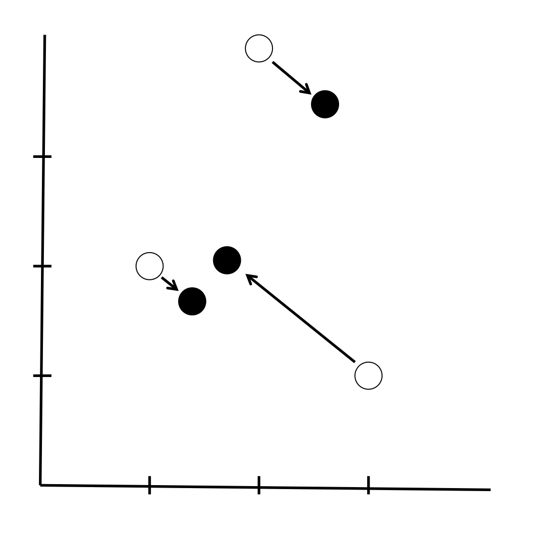
We can calculate the coordinates of our new embedding (the black points) as
This is somewhat absurd when our new embedding has rank 1, but it shows that the black points that was at (1, 2) moves to a position 2.19 along the rank 1 subspace, the point that was at (2, 4) moves to a position 4.39 along this line, and the point that was at (3, 1) moves to a position 2.62 along this line. You can imagine that this new basis for the subspace we have created is of more use when the new embedding is of (much) higher rank than 1.
We could equivalently view our system as being the coordinates of terms in 3-dimensional document space. In this case our svd reduces this space to an equivalent rank 1 subspace, and in this space the terms are located at
Additionally, this allows us to derive an equation describing the line of which the black points in the diagram sit - it is y = (4.41 / 3.38) x.
Finally, note that in terms of being an algorithm that
- uses matrix algebra; and
- results in the creation of a reduced-rank subspace; which
- is somehow closest to the original space; and
- has a basis that is a linear combination of the original basis vectors
SVD is clearly similar in ethos to principal component analysis. Obviously the two can be formally compared.
The point of all this madness
Deep breath now, the hardcore (well, first year Linear Algebra course, which is hard for me) maths is done. We can now see the point of all this.
First, a recap:
- We defined an initial embedding for our documents based on the words that remained in the vocabulary after we had done our feature selection, and using some sort of weighting scheme of our choice.
- We did some
magicLinear Algebra to reduce the rank of our initial embedding so that all our our documents now lie on some sort of k-dimensional hyperplane.
Why is this good? Take a look at the diagram above again. The black points lie on a line. They are the best one-dimensional approximation to our 2-dimensional original embedding. If we think that there is random noise in our system (e.g. there is an element of chance in what words appear in our document even once their actual topical content is determined), we might say that we should approximate the system by the line on which the black points sit, so that our real data (the white points) is made up of the black points (the signal) plus some noise term.
We might say that, once we take randomness out of the picture, the points that end up closer to one another are “truly” closer in information content than ones that end up far away. Reducing the dimensionality gives us a model that doesn’t overfit - in particular, it doesn’t take synonyms as being separate entities, but (at least hopefully) sees them as meaning similar things (because synonyms will tend to co-occur with similar terms).
The bottom line
Once you’ve got your rank-k subspace, and the coordinates of your new embedding on this k-dimensional hyperplane, you can do your similarity measure on this and do Search and also clustering to do Topics.
But wait: how do we choose k?
Choosing the value of k is not necessarily simple. If you pick k too large then you risk paying too much attention to outliers like rare words; this is conceptually similar to overfitting. If you pick k too small then you risk throwing away too much information.
There are doubtless statistical measures one can choose to see how well a rank-k approximation fits the original rank-r subspace for each choice of k, and then looking for a tell-tale elbow in a plot of this, or something. However, these optimisation techniques assume we’re trying to strike a balance between computational efficiency (lowering k) and fidelity to the original space (raising k). But we’re also concerned that the original space contains noise, and in some sense we’re looking for a ‘best fit’ to some latent ‘true’ distribution for the documents.
Consequently we have so far used trial and error to determine k and not worried too much about needing to be incredibly precise. The important thing is to find a value of k that gives the end user something that seems meaningful and useful.
Similarity measures
The standard similarity measure to use when comparing embedded documents is cosine similarity. In practice everyone seems to use this.
In actual fact we always (re)normalise our embedding so that everything is on a hypersphere: under these circumstances (I think) Euclidean distance and [cosine similarity](Glossary.md#cossim are equivalent.
Final note: potential problems
Writing this has allowed me to think about our process in more detail, and I am aware that there are potentially some issues with it. In practice it works fine in the Parliamentary Analysis Tool, so I’m not too worried. But if anyone knows the answers to the following questions we might be able to do better (or at least set things on a firmer mathematical grounding).
The process we follow goes
- Embed our documents in a vector space of degree N, where N is the size of our vocabulary. The initial embedding will be of rank r where r ≤ N: this means that within our N-dimensional vector space, our documents sit on a hyperplane of dimension r.
- Normalise our document vectors so that they all have unit length. Following this step, the documents sit on a hypersphere of dimension (r - 1) within our N-dimensional vector space. Although we must have thrown away information here, we have conserved the angle between document vectors, so we don’t mind.
- Reduce the rank of our embedding to rank k by using SVD, where we choose some k ≤ r - 1. Following this step our documents sit on a k-dimensional hyperplane. Their new positions are determined so as to move them as little as possible from their previous positions on the (r - 1)-sphere. To be precise the total squared distance that they all move is minimised. However, notice that we have not minimised changes in the angles between them, which is what we’re actually interested in.
- Normalise again, so that our documents now sit on a (k - 1)-dimensional hypersphere. Again, this normalisation conserves the angles between the documents.
The problem is that we are playing fast and loose with what we are trying to conserve or minimise. In steps 2 and 4 we are happy to normalise because we are concerned with angles between vectors, and not Euclidean distances. But at step 3 we use a low-rank approximation that minimises the (total squared) Euclidean distance between the new points and the original points. This is inconsistent, at best.
As I say, in practice it seems like the results are still fine, but if anyone knows how to produce a low-rank approximation that minimises changes to angles between points, and can implement it in R, I would be a lot happier.
It might be equivalent (or perhaps: better) to be able to find the optimal k-dimensional hyperspherical approximation to data which sits on an r-dimensional hypersphere. These people have done this, but I haven’t looked at implementing it in R. Their first definition of ‘optimal’, the ‘Fidelity test’ seems like it would be appropriate in our case.
Written by Sam Tazzyman, DaSH, MoJ